MS EXCEL: TWO-DIMENSIONAL LOOKUP 

This Excel tutorial explains how to perform a two-dimensional lookup (with screenshots and step-by-step instructions). This is example #1.

Question: I'm trying to reference a particular cell within an xy axis chart and can't find the formula or function that allows me to do so.

For example A1 needs to equal where row 12 intersects column F on a chart.

I know the lookup function can get me a value from a known array of values located in the corresponding column, but I can't get it to figure from an array of columns. Can you help?

Answer: In effect, what we are trying to do is perform a 2-dimensional lookup in Excel. To find a value in Excel based on both a column and row value, you will need to use both a vlookup function and a match function.

Let's look at an example to see how you would use this function in a worksheet:

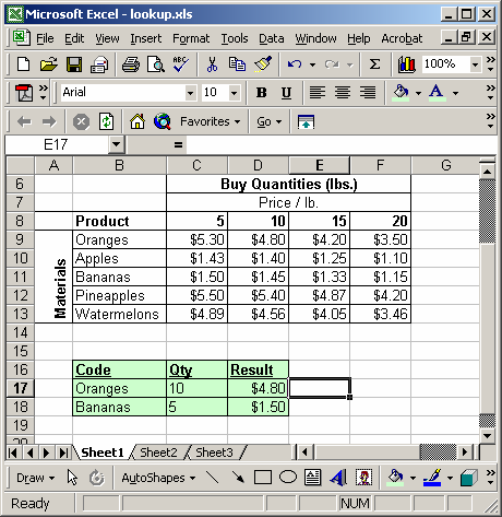
In the spreadsheet above, we have a listing of products (Oranges, Apples, Bananas, Pineapples, Watermelons) and a listing of quantity columns (5 lbs, 10 lbs, 15 lbs, and 20 lbs). What we want to do is find the correct value based on a product and quantity combination.

In the first case, we want to find the price/lb for 10 lbs of oranges. To find the price/lb, we've entered the following formula into cell D17:

=VLOOKUP(B17, $B$8:$F$13, MATCH(C17, $B$8:$F$8, 0), FALSE)

This formula returns the value of $4.80.

In the second example, we are looking for the price/lb for 5 lbs of bananas. We've entered the following formula into cell D18:

=VLOOKUP(B18, $B$8:$F$13, MATCH(C18, $B$8:$F$8, 0), FALSE)

This formula returns the value of $1.50